The random field is a significant concept with diverse applications, especially in geotechnical engineering. When dealing with soil layers, there is often limited information available regarding the distribution of soil characteristics within the soil profile. Consequently, accurately modeling the current state of the soil may prove difficult. In such scenarios, a viable solution is to employ a random field to represent the spatial variability of soil characteristics in a random fashion.
However, the implementation of a random field can be complex, which can pose challenges for its practical application. In this blog post, we will present a simple example and guide you through the process step by step to demonstrate how a random field can be implemented in MATLAB. This example can serve as an introductory exercise to help you become familiar with random fields and the main parameters that influence them.
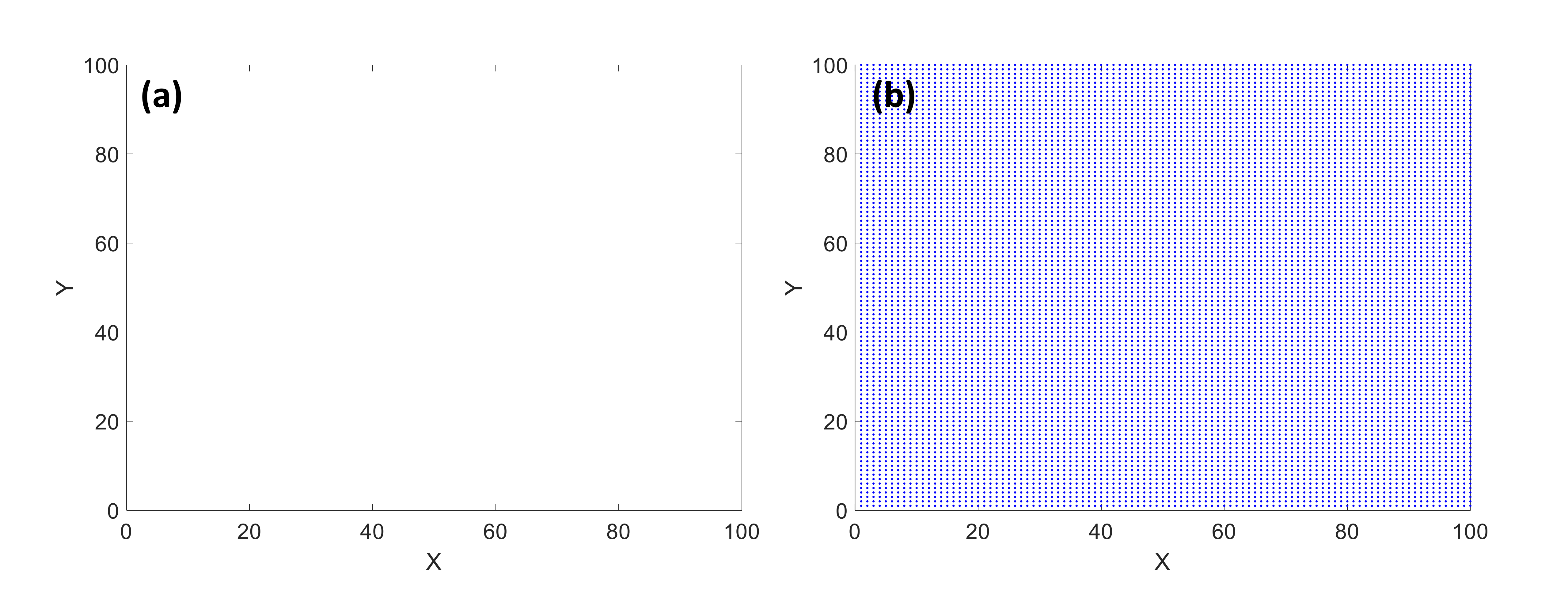
Imagine we have a square section of soil layer that is 100 meters wide and 100 meters deep (Figure 1a). Our goal is to generate a random field realization within this area.

Figure 1: The region for generating the random field: (a) size and dimensions of the region; (b) generated grid points
The first step is to divide the entire region into grids or meshes to assign random values. Let’s divide the area into 100 grids in the X direction and 100 grids in the Y direction. This division can be outlined as follows:
nx = 100;
ny = 100;
Next, we will determine the correlation length and variance. The correlation length is a key parameter in random field analysis, indicating the extent of similarity between adjacent points. A larger correlation length results in broader regions of similarity, while a smaller correlation length leads to more localized similarities. For this scenario, we will set the correlation length to 10 meters and the variance to 1.
cl = 10;
variance = 1;
We can now generate the grids within the designated region by using the ‘meshgrid’ command. The results will be stored in two vectors, x and y.
[x,y] = meshgrid(1:nx,1:ny);
After running the code up to this point, the vectors x and y have been created. To visualize the grid points, we can plot x versus y on a graph as follows:
Plot(x,y,’.’,color = ‘b’)
The output is presented in figure 1b, showing 100 grid points in the x and y directions. Next, we will generate a random value corresponding to each of these grid points. This will be done using a standard normal distribution, as outlined below:
random_f = variance*randn(nx,ny);
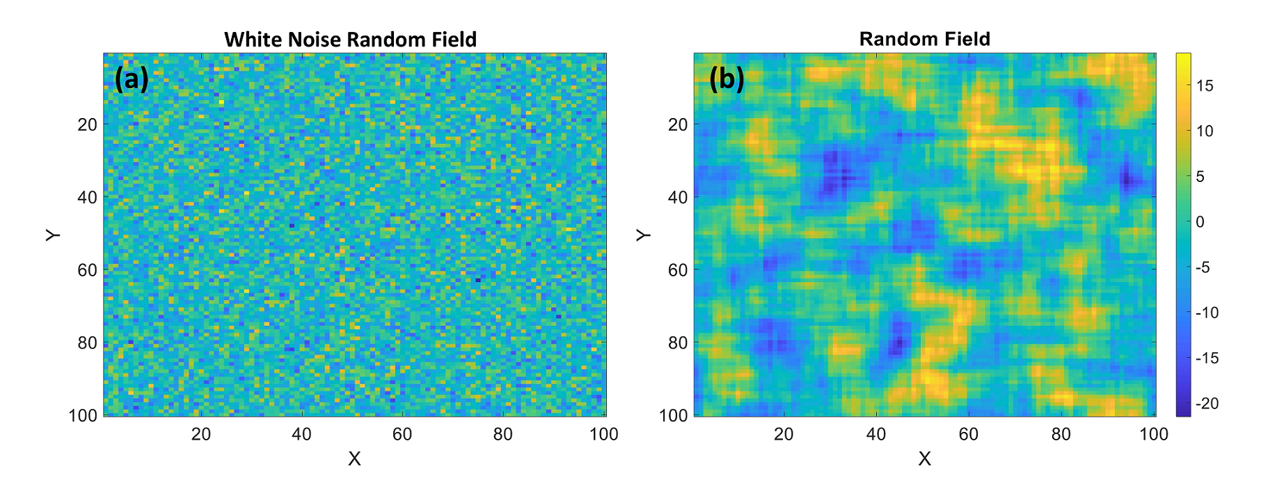
This is a preliminary version of the random field generated from independent standard normal values, hence it is termed as a white noise random field. We can visualize this random field using a contour plot. The result is depicted in Figure 2a.
imagesc(random_f)

Figure 2: Random field realization (a) white noise random field (b) correlation length = 10 m
In this random field, each point is independent of its neighboring points, resulting in significant variations between adjacent points. However, this does not reflect the reality of soil profiles, where we typically find regions with similar characteristics. To address this discrepancy, we need to introduce a correlation function into the white noise random field. This correlation function is defined as:
corr_f = exp(-((x-x(1)).^2+(y-y(1)).^2)/cl.^2);
This process yields a 100x100 matrix illustrating the correlation function. The next step is to convolve this matrix with the white noise random field created earlier. Various techniques have been suggested in the literature for this task. The method we are utilizing involves transforming both matrices into the frequency domain using the fast Fourier transform. In the frequency domain, convolution simplifies to a basic multiplication operation. Once the convolution process is completed, we revert the result back to the original domain using the inverse fast Fourier transform. This computation can be executed in Matlab as detailed below:
random_f = real(ifft2(fft2(random_f).*fft2(corr_f)));
As noted, we only consider the real part of the result. Any imaginary components in the inverse fast Fourier transform are disregarded. With the random field now updated, the next task is to visualize it. This can be accomplished by creating a contour plot, as outlined below:
%% Plot the random field
figure(1)
imagesc(random_f)
colorbar
title('Random Field')
xlabel('X')
ylabel('Y')
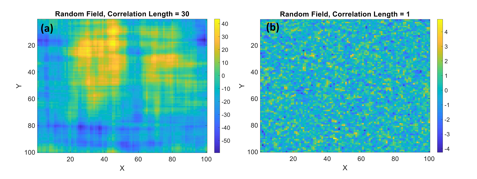
The results are illustrated in Figure 2b, revealing distinct regions with similar characteristics within the random field. This indicates successful generation of the random field in the desired area. To further analyze the influence of correlation length on the overall shape of the random field, we conducted additional iterations with correlation lengths of 30 and 1. The outcomes are presented in Figures 3a and 3b, respectively.

Figure 3: Random field realizations with (a) correlation length = 30 m and (b) correlation length = 1 m
It is evident that as the correlation length increases, the so-called similar regions also expand in size. Conversely, with a smaller correlation length, these similar regions shrink significantly, leading the random field to closely resemble a white noise random field.
Another important point to note is that the correlation length can vary in different directions. This means that we can have distinct correlation lengths in the X and Y directions, as illustrated below:
cl_x = 10;
cl_y = 30;
Subsequently, we can integrate them into the correlation function in the following manner:
corr_f = exp(-((x-x(1)).^2/cl_x.^2+(y-y(1)).^2/cl_y.^2));
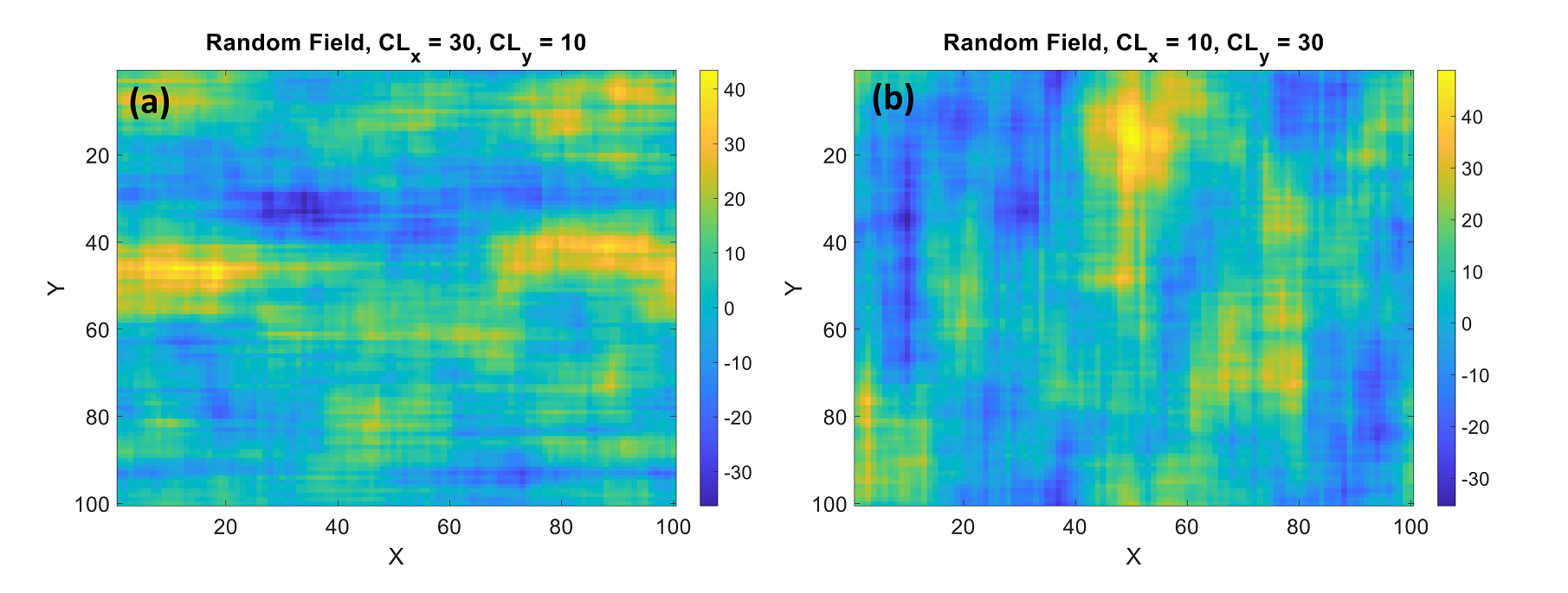
Next, we conduct the model with two scenarios: one where cl_x is greater than cl_y, and the other where cl_y is greater than cl_x. The results are presented in Figures 4a and 4b.

Figure 4: Random field realizations with different correlation lengths in X and Y directions (a) CLx = 30 m and CLy = 10 m and (b) CLx = 10 m and CLy = 30 m
Observing the results, it is evident that when the correlation length in the X direction is greater, the corresponding regions exhibit a slight stretching in the X direction. Conversely, when the correlation length in the Y direction is larger, the related regions are stretched in the Y direction. Therefore, the correlation length plays a crucial role in shaping the random field and aligning it more closely with reality.
This marks the conclusion of the blog post. For those seeking further insights and detailed explanations on the subject matter covered in this post, a training video conducted by Dr. Mahdi Shadabfar is available for viewing. You can access the video by clicking on the provided link below:
